Closed-form Solution for the Fibonacci Sequence
Fibonacci sequence recurrence relation is a second-order difference equation:
\[f[n] = f[n-1] + f[n-2]\]With initial conditions \(f[0]=0\) and \(f[1]=1\), this yields the familiar Fibonacci sequence: {0, 1, 1, 2, 3, 5, 8, 13, 21, 34, 55, 89, 144, 233, 377, 610, 987, …}. You might find it intriguing for its various roles in nature (or not).
But how do we go about calculating, say, the 1000th number in the Fibonacci sequence? Chug through the sequence from the beginning? or is there a closed-form solution?
How about:
\[\begin{align*} f_n &= \text{round}\left(\frac{\sqrt{5}}{5}{\left(\frac{1+\sqrt{5}}{2}\right)}^n\right) \cr \end{align*}\]{0, 1, 1, 2, 3, 5, 8, 13, 21, 34, 55, 89, 144, 233, 377, 610, 987, 1597, 2584, 4181, 6765, …}
I wrote this page mostly as a review for myself of two methods for solving linear constant coefficient ordinary difference equations, using my favorite example. It doesn’t explain in detail what an eigenvalue or a z-transform is, though. Also, the Wikipedia Fibonacci number page touches on the linear algebra derivation below, but does not go into much depth.
The Fibonacci sequence is usually defined to start with {0, 1, 1, 2, …} from n=0. However, I use initial conditions \(f[-1]=0\) and \(f[0]=1\) below, to make things line up easily between the linear algebra and z-transform approaches. This means that the Fibonacci sequences calculated below start with {1, 1, 2, 3, 5, …} from n=0, which is simply shifted by one step in time from {0, 1, 1, 2, 3, 5, …}. I’ll account for this and get back to the sequence starting with 0 at n=0 in the third section.
Linear Algebra Way
We can rewrite the original recurrence relation as:
\[f[n+1] = f[n] + f[n-1]\]and then assign variables \(f_n = f[n]\) and \(f_{n-1} = f[n-1]\). So \(f_n\) holds the current value, and \(f_{n-1}\) holds the past value. Combined, they constitute the information required to compute the next value of the sequence, or equivalently, they represent the state of the system at any given time.
Now we can easily recast the recurrence relation in matrix form as a system of coupled first-order difference equations, capturing how these two dependent variables evolve over time:
\[\begin{align*} \begin{bmatrix} f_{n}[n+1] \cr f_{n-1}[n+1] \end{bmatrix} = \begin{bmatrix} 1 & 1 \cr 1 & 0 \end{bmatrix} \begin{bmatrix} f_{n}[n] \cr f_{n-1}[n] \end{bmatrix} \cr \end{align*}\]The first equation, \(f_n[n+1] = f_n[n] + f_{n-1}[n]\), is a restatement of the recurrence relation, but in terms of the two separate variables \(f_n\) and \(f_{n-1}\) holding the current and past value, respectively. The second equation in the system, \(f_{n-1}[n+1] = f_{n}[n]\), is a trivial statement, but necessary to characterize the evolution of the second variable \(f_{n-1}\).
This also can be thought of as a DT state space model of the system, with state vector \(\vec{q}\), and state transition matrix \(\mathbf{A}\):
\[\begin{align*} \vec{q}\,[n] &= \begin{bmatrix} f_n \cr f_{n-1} \end{bmatrix} \cr \vec{q}\,[n+1] &= \mathbf{A} \vec{q}\,[n] \cr \vec{q}\,[n+1] &= \begin{bmatrix} 1 & 1 \cr 1 & 0 \end{bmatrix} \vec{q}\,[n] \end{align*}\](Notation note: \(\vec{q}\) is a column vector, \(\mathbf{A}\) is an 2 x 2 matrix, \(\lambda\) is a scalar.)
First, let’s give iterative computation of the Fibonacci sequence a try.
Define initial conditions with the first two numbers of the Fibonacci sequence:
\[\vec{q}\,[0] = \begin{bmatrix} f_0 \cr f_{-1} \end{bmatrix} = \begin{bmatrix} 1 \cr 0 \end{bmatrix}\]Iteratively compute up to \(\vec{q}\,[4]\):
\[\begin{align*} \vec{q}\,[0] &= \begin{bmatrix} 1 \cr 0 \end{bmatrix} \cr \vec{q}\,[1] = \mathbf{A} \vec{q}\,[0] = \begin{bmatrix} 1 & 1 \cr 1 & 0 \end{bmatrix} \begin{bmatrix} 1 \cr 0 \end{bmatrix} &= \begin{bmatrix} 1 \cr 1 \end{bmatrix} \cr \vec{q}\,[2] = \mathbf{A} \vec{q}\,[1] = \begin{bmatrix} 1 & 1 \cr 1 & 0 \end{bmatrix} \begin{bmatrix} 1 \cr 1 \end{bmatrix} &= \begin{bmatrix} 2 \cr 1 \end{bmatrix} \cr \vec{q}\,[3] = \mathbf{A} \vec{q}\,[2] = \begin{bmatrix} 1 & 1 \cr 1 & 0 \end{bmatrix} \begin{bmatrix} 2 \cr 1 \end{bmatrix} &= \begin{bmatrix} 3 \cr 2 \end{bmatrix} \cr \vec{q}\,[4] = \mathbf{A} \vec{q}\,[3] = \begin{bmatrix} 1 & 1 \cr 1 & 0 \end{bmatrix} \begin{bmatrix} 3 \cr 2 \end{bmatrix} &= \begin{bmatrix} 5 \cr 3 \end{bmatrix} \cr \end{align*}\]Notice the familiar Fibonacci sequence sitting in the \(f_n\) element of the \(\vec{q}\) state vector: {1, 1, 2, 3, 5}.
From above, it follows that we can also compute \(\vec{q}\,[4]\) directly, by exponentiating the transition matrix:
\[\begin{align*} \vec{q}\,[4] &= {\begin{bmatrix} 1 & 1 \cr 1 & 0 \end{bmatrix}}{\begin{bmatrix} 1 & 1 \cr 1 & 0 \end{bmatrix}}{\begin{bmatrix} 1 & 1 \cr 1 & 0 \end{bmatrix}}{\begin{bmatrix} 1 & 1 \cr 1 & 0 \end{bmatrix}} \vec{q}\,[0] = \begin{bmatrix} 5 \cr 3 \end{bmatrix} \cr \vec{q}\,[4] &= {\begin{bmatrix} 1 & 1 \cr 1 & 0 \end{bmatrix}}^4 \vec{q}\,[0] = \begin{bmatrix} 5 \cr 3 \end{bmatrix} \cr \vec{q}\,[4] &= {\mathbf{A}}^4 \vec{q}\,[0] = \begin{bmatrix} 5 \cr 3 \end{bmatrix} \cr \end{align*}\]But, exponentiating a matrix can be expensive, and we can do better than this. In a sense, we can evolve in the “natural direction” of the system to reduce the required computation. We can do this with an eigendecomposition of the state transition matrix \(A\).
By definition of eigenvalue \(\lambda\) and eigenvector \(\vec{v}\):
\[\mathbf{A}\vec{v} = \lambda \vec{v}\]To represent all eigenvalues and eigenvectors of \(\mathbf{A}\) (assuming 2x2), we can organize the statement above as:
\[\begin{align*} \begin{bmatrix} \mathbf{A} \vec{v_1} & \mathbf{A} \vec{v_2} \end{bmatrix} &= \begin{bmatrix} \lambda_1 \vec{v_1} & \lambda_2 \vec{v_2} \end{bmatrix} \cr \mathbf{A} \begin{bmatrix} \vec{v_1} & \vec{v_2} \end{bmatrix} &= \begin{bmatrix} \vec{v_1} & \vec{v_2} \end{bmatrix} \begin{bmatrix} \lambda_1 & 0 \cr 0 & \lambda_2 \end{bmatrix} \cr \mathbf{A} \mathbf{V} &= \mathbf{V} \mathbf{\Lambda} \cr \end{align*}\]Then we can rewrite \(\mathbf{A}\) in terms of its eigenvalues and eigenvectors:
\[\begin{align*} \mathbf{A} &= \mathbf{V} \mathbf{\Lambda} {\mathbf{V}}^{-1} \end{align*}\]Why bother with this representation of \(\mathbf{A}\)? Well, it leads to a particularly useful simplification to exponentiating \(\mathbf{A}\), which we need to do to compute the next value of the Fibonacci sequence. It also reveals the characteristics of \(\mathbf{A}\) that are relevant to how this sequence evolves.
\[\begin{align*} {\mathbf{A}}^n &= (\mathbf{V} \mathbf{\Lambda} {\mathbf{V}}^{-1})^n \cr {\mathbf{A}}^n &= (\mathbf{V} \mathbf{\Lambda} {\mathbf{V}}^{-1}) (\mathbf{V} \mathbf{\Lambda} {\mathbf{V}}^{-1}) (\mathbf{V} \mathbf{\Lambda} {\mathbf{V}}^{-1}) \cdots \cr {\mathbf{A}}^n &= \mathbf{V} \mathbf{\Lambda} ({\mathbf{V}}^{-1} \mathbf{V}) \mathbf{\Lambda} ({\mathbf{V}}^{-1} \mathbf{V}) \mathbf{\Lambda} ({\mathbf{V}}^{-1} \cdots \cr {\mathbf{A}}^n &= \mathbf{V} \mathbf{\Lambda} \mathbf{\Lambda} \mathbf{\Lambda} \cdots {\mathbf{V}}^{-1} \cr {\mathbf{A}}^n &= \mathbf{V} {\mathbf{\Lambda}}^n {\mathbf{V}}^{-1} \cr {\mathbf{A}}^n &= \mathbf{V} \begin{bmatrix} {\lambda_1}^n & 0 \cr 0 & {\lambda_2}^n \end{bmatrix} {\mathbf{V}}^{-1} \cr \end{align*}\]To calculate the nth element of Fibonacci sequence, exponentiating the matrix \(\mathbf{A}\) has been reduced to exponentiating its scalar eigenvalues \(\lambda_1\), \(\lambda_2\).
To exercise this, let’s find the eigenvalues and eigenvectors of \(\mathbf{A}\):
\[\begin{align*} \mathbf{A}\vec{v} &= \lambda \vec{v} \cr \mathbf{A}\vec{v} - \lambda \vec{v} &= 0 \cr (\mathbf{A} - \lambda\mathbf{I})\vec{v} &= 0 \cr \det{(\mathbf{A} - \lambda\mathbf{I})} &= 0 \cr \end{align*}\] \[\begin{align*} \det\left({\begin{bmatrix} 1-\lambda & 1 \cr 1 & 0-\lambda \end{bmatrix}}\right) &= 0 \cr -\lambda + {\lambda}^2 - 1 &= 0 \cr {\lambda}^2 - \lambda - 1 &= 0 \cr \end{align*}\]Eigenvalues:
\[\begin{align*} \lambda &= \frac{1 \pm \sqrt{1+4}}{2} \cr \lambda_1 &= \frac{1+\sqrt{5}}{2} = 1.61803399 \ldots \cr \lambda_2 &= \frac{1-\sqrt{5}}{2} = -0.618033989 \ldots \cr \end{align*}\]Eigenvectors:
\[\begin{align*} \begin{bmatrix} 1-\lambda & 1 \cr 1 & -\lambda \end{bmatrix} \begin{bmatrix} x_1 \cr x_2 \end{bmatrix} &= 0 \cr x_1 - \lambda x_2 &= 0\cr x_1 &= \lambda x_2 \cr \text{Pick $x_2$ = 1} \cr \end{align*}\] \[\begin{align*} \vec{v}_1 &= \begin{bmatrix} \frac{1+\sqrt{5}}{2} \cr 1 \end{bmatrix} \cr \vec{v}_2 &= \begin{bmatrix} \frac{1-\sqrt{5}}{2} \cr 1 \end{bmatrix} \cr \end{align*}\]Eigenvalues \(\lambda_1\) and \(\lambda_2\) are the natural frequencies or the poles of the system governed by \(\mathbf{A}\). \(\lambda_1\) is also the Golden Ratio.
Now we can rewrite the evolution of state vector \(\vec{q}\) in terms of the eigendecomposition of state transition matrix \(\mathbf{A}\):
\[\begin{align*} \vec{q}\,[n+1] &= \mathbf{A} \vec{q}\,[n] \cr \vec{q}\,[n+1] &= \mathbf{V} \mathbf{\Lambda} {\mathbf{V}}^{-1} \vec{q}\,[n] \cr \vec{q}\,[n+1] &= \begin{bmatrix} \vec{v}_1 \vec{v}_2 \end{bmatrix} \begin{bmatrix} \lambda_1 & 0 \cr 0 & \lambda_2 \end{bmatrix} {\begin{bmatrix} \vec{v}_1 \vec{v}_2 \end{bmatrix}}^{-1} \vec{q}\,[n] \cr \vec{q}\,[n+1] &= \begin{bmatrix} \frac{1+\sqrt{5}}{2} & \frac{1-\sqrt{5}}{2} \cr 1 & 1 \end{bmatrix} \begin{bmatrix} \frac{1+\sqrt{5}}{2} & 0 \cr 0 & \frac{1-\sqrt{5}}{2} \end{bmatrix} {\begin{bmatrix} \frac{1+\sqrt{5}}{2} & \frac{1-\sqrt{5}}{2} \cr 1 & 1 \end{bmatrix}}^{-1} \vec{q}\,[n] \end{align*}\]Let’s get that matrix inverse \({\mathbf{V}}^{-1}\) out of the way:
\[\begin{align*} {\begin{bmatrix} \frac{1+\sqrt{5}}{2} & \frac{1-\sqrt{5}}{2} \cr 1 & 1 \end{bmatrix}}^{-1} &= \begin{bmatrix} \frac{\sqrt{5}}{5} & \frac{5-\sqrt{5}}{10} \cr \frac{-\sqrt{5}}{5} & \frac{5+\sqrt{5}}{10} \end{bmatrix} \end{align*}\]So, we have:
\[\begin{align*} \vec{q}\,[n+1] &= \begin{bmatrix} \frac{1+\sqrt{5}}{2} & \frac{1-\sqrt{5}}{2} \cr 1 & 1 \end{bmatrix} \begin{bmatrix} \frac{1+\sqrt{5}}{2} & 0 \cr 0 & \frac{1-\sqrt{5}}{2} \end{bmatrix} \begin{bmatrix} \frac{\sqrt{5}}{5} & \frac{5-\sqrt{5}}{10} \cr \frac{-\sqrt{5}}{5} & \frac{5+\sqrt{5}}{10} \end{bmatrix} \vec{q}\,[n] \cr \end{align*}\]This is cool, because if we manipulate this further it leads to a closed-form solution for the nth element of the Fibonacci sequence.
To do this, let’s rewrite \(\vec{q}\,[n]\) in terms of the initial conditions \(\vec{q}\,[0]\), just as we did with \(\vec{q}\,[4]\) above:
\[\begin{align*} \vec{q}\,[n] &= \mathbf{V} {\mathbf{\Lambda}}^n {\mathbf{V}}^{-1} \vec{q}\,[0] \cr \vec{q}\,[n] &= \begin{bmatrix} \frac{1+\sqrt{5}}{2} & \frac{1-\sqrt{5}}{2} \cr 1 & 1 \end{bmatrix} \begin{bmatrix} {\lambda_1}^n & 0 \cr 0 & {\lambda_2}^n \end{bmatrix} \begin{bmatrix} \frac{\sqrt{5}}{5} & \frac{5-\sqrt{5}}{10} \cr \frac{-\sqrt{5}}{5} & \frac{5+\sqrt{5}}{10} \end{bmatrix} \begin{bmatrix} 1 \cr 0 \end{bmatrix} \cr \vec{q}\,[n] &= \begin{bmatrix} \frac{1+\sqrt{5}}{2} & \frac{1-\sqrt{5}}{2} \cr 1 & 1 \end{bmatrix} \begin{bmatrix} {\lambda_1}^n & 0 \cr 0 & {\lambda_2}^n \end{bmatrix} \begin{bmatrix} \frac{\sqrt{5}}{5} \cr \frac{-\sqrt{5}}{5} \end{bmatrix} \cr \vec{q}\,[n] &= \begin{bmatrix} \frac{1+\sqrt{5}}{2} & \frac{1-\sqrt{5}}{2} \cr 1 & 1 \end{bmatrix} \begin{bmatrix} \frac{\sqrt{5}}{5}{\lambda_1}^n \cr \frac{-\sqrt{5}}{5}{\lambda_2}^n \end{bmatrix} \cr \vec{q}\,[n] &= \begin{bmatrix} \frac{5+\sqrt{5}}{10}{\lambda_1}^n + \frac{5-\sqrt{5}}{10}{\lambda_2}^n \cr \frac{\sqrt{5}}{5}{\lambda_1}^n - \frac{\sqrt{5}}{5}{\lambda_2}^n \end{bmatrix} \cr \end{align*}\]We defined the state vector \(\vec{q}\) as \(\begin{bmatrix} f_n \cr f_{n-1} \end{bmatrix}\), and now we have closed-form solutions for how \(\vec{q}\), containing both \(f_n\) and \(f_{n-1}\), evolves over time. But, we really only need the top element, \(f_n\), from the above closed-form evolution of \(\vec{q}\) to compute the whole Fibonacci sequence.
\[\begin{align*} f_n &= \frac{5+\sqrt{5}}{10}{\lambda_1}^n + \frac{5-\sqrt{5}}{10}{\lambda_2}^n \cr f_n &= \frac{5+\sqrt{5}}{10}{\left(\frac{1+\sqrt{5}}{2}\right)}^n + \frac{5-\sqrt{5}}{10}{\left(\frac{1-\sqrt{5}}{2}\right)}^n \cr f_n &\approx 0.723606798 \cdot (1.61803399)^n + 0.276393202 \cdot (-0.618033989)^n \end{align*}\]Let’s tabulate a few values of the Fibonacci sequence using our closed-form expression for it. Here is a link to the exact expression in Wolfram-Alpha here. At the bottom, you will find: {1, 1, 2, 3, 5, 8, 13, 21, 34, 55, 89, 144, 233, 377, 610, 987, 1597, 2584, 4181, 6765, 10946}.
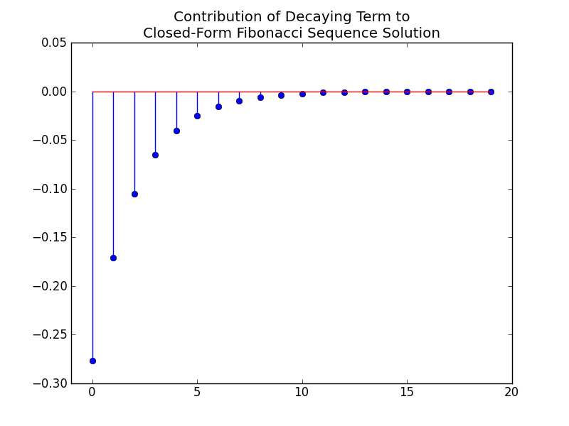
If we look closely at our solution, we can see that the second mode associated with \(\lambda_2\) (that is, the \(+ \frac{5-\sqrt{5}}{10}{\left(\frac{1-\sqrt{5}}{2}\right)}^n\)) is a decaying mode, since \(\lvert \lambda_2 \rvert = 0.618 < 1\); and the first mode associated with \(\lambda_1\) is a growing mode, since \(\lvert \lambda_1 \rvert = 1.618 > 1\). This makes sense since we are exponentiating these eigenvalues in our closed-form solution.
import pylab
import numpy
n = numpy.arange(0, 20)
decay = 0.276393202*(-0.618033989**n)
pylab.stem(n, decay)
pylab.xlim(-1, 20)
pylab.title("Contribution of Decaying Term to\nClosed-Form Fibonacci Sequence Solution")
pylab.show()
By n=11, the contribution from the second term is \(0.276393202 \cdot (-0.618033989)^{11} \approx -0.001\). We can form an even simpler approximation for computing the Fibonacci sequence by neglecting this term associated with \(\lambda_2\).
This leaves us with:
\[\begin{align*} f_n &\approx \frac{5+\sqrt{5}}{10}{\left(\frac{1+\sqrt{5}}{2}\right)}^n \end{align*}\]Let’s check the values of the approximated version on Wolfram-Alpha here. We get the values: {0.723607, 1.17082, 1.89443, 3.06525, 4.95967, 8.02492, 12.9846, 21.0095, 33.9941, 55.0036, 88.9978, 144.001, 232.999, 377.001, 610., 987., 1597., 2584., 4181., 6765., 10946.}.
These are obviously not the exact Fibonacci sequence integer values, but if we throw a round() into the expression, we can recover the exact values. This is because the second term we discarded is always less than 0.5 in magnitude (we can check its maximum at n=0 -> -0.276393202, also illustrated in the plot above). Therefore, its missing contribution is never large enough to cause round() to round the simplified expression up or down to an integer not in the sequence.
Our final closed-form solution to the Fibonacci sequence:
\[\begin{align*} f_n &= \text{round}\left(\frac{5+\sqrt{5}}{10}{\left(\frac{1+\sqrt{5}}{2}\right)}^n\right) \cr \end{align*}\]Once again, we can check on Wolfram-Alpha here and see that we get the correct sequence: {1, 1, 2, 3, 5, 8, 13, 21, 34, 55, 89, 144, 233, 377, 610, 987, 1597, 2584, 4181, 6765, 10946, …}.
Z-Transform Way
An alternate approach to yielding the same closed-form solution is to use z-transforms and inverse z-transforms.
Let’s add an input signal to the original difference equation. As before, we’ll load the system with the same initial conditions, but we’ll use the input signal to “deliver them” with an impulse, \(x[n] = \delta[n]\), and it will make manipulation easier here. Since \(x[n]\) is taking care of the initial conditions, we assume \(y[n]\) starts at rest.
\[y[n] = y[n-1] + y[n-2] + x[n]\]\(x[n]=\delta[n]\) above implies that \(y[-1] = 0\) and \(y[0] = 1\), which is effectively the same initial conditions as we stated above, namely \(f_{-1} = 0\) and \(f_0 = 1\).
Taking the z-transform of the difference equation:
\[Y(z) = z^{-1}Y(z) + z^{-2}Y(z) + X(z)\]And solving for the transfer function, \(\frac{Y(z)}{X(z)}\):
\[\begin{align*} Y(z)(1 - z^{-1} - z^{-2}) &= X(z) \cr \end{align*}\] \[\begin{align*} \frac{Y(z)}{X(z)} &= \frac{1}{1 - z^{-1} - z^{-2}} \cr \frac{Y(z)}{X(z)} &= \frac{z^{2}}{z^{2} - z - 1} \end{align*}\]Now let’s factor the denominator of the transfer function, so we can do a partial fraction expansion:
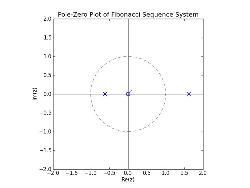
\[\begin{align*} z^{2} - z - 1 &= 0 \cr \end{align*}\] \[\begin{align*} z &= \frac{1 \pm \sqrt{5}}{2} \cr \end{align*}\] \[\begin{align*} z^{2} - z - 1 &= (z - \frac{1+\sqrt{5}}{2})(z - \frac{1-\sqrt{5}}{2}) \cr \end{align*}\]Naturally (pun intended), the poles of this system, \(z_1 = \frac{1+\sqrt{5}}{2}\) and \(z_2 = \frac{1-\sqrt{5}}{2}\), are the same eigenvalues \(\lambda_1\) and \(\lambda_2\) we found above. Just as before, but in the signals and systems sense, \(z_2\) is inside the unit circle (\(\lvert z_2 \rvert < 1\)), so the mode associated with it is a decaying mode; and \(z_1\) is outside the unit circle (\(\lvert z_1 \rvert > 1\)), so the mode associated with it is a growing mode.
import pylab
import numpy

zeros = numpy.array([0+0j, 0+0j])
poles = numpy.array([1.61803399+0j, -0.618033989+0j])

circle = pylab.Circle((0,0), radius=1, fc='white', linestyle='dashed', color='gray')
pylab.plot(numpy.real(zeros), numpy.imag(zeros), 'o', markeredgecolor='blue', markerfacecolor='white', markersize=8, markeredgewidth=1.25)
pylab.plot(numpy.real(poles), numpy.imag(poles), 'bx', markersize=8, markeredgewidth=1.25)
pylab.xlim(-2, 2)
pylab.ylim(-2, 2)
pylab.gca().add_patch(circle)
pylab.gca().set_aspect(1)
pylab.text(0.05, 0.05, '2', fontsize=7, color='blue')
pylab.axhline(color='black')
pylab.axvline(color='black')
pylab.xlabel('Re(z)')
pylab.ylabel('Im(z)')
pylab.title('Pole-Zero Plot of Fibonacci Sequence System')
pylab.show()
Transfer function with the factored denominator:
\[\begin{align*} \frac{Y(z)}{X(z)} &= \frac{z^{2}}{(z - \frac{1+\sqrt{5}}{2})(z - \frac{1-\sqrt{5}}{2})} \cr \end{align*}\]Now carrying out the partial fraction expansion:
\[\begin{align*} \frac{z^2}{(z-\lambda_1)(z-\lambda_2)} &= \frac{A z}{z-\lambda_1} + \frac{B z}{z-\lambda_2} \cr z^2 &= A z (z-\lambda_2) + B z (z-\lambda_1) \cr \end{align*}\] \[\begin{align*} z^2 &= A z^2 + B z^2 \cr 0 &= - A z \lambda_2 - B z \lambda_1 \cr \end{align*}\] \[\begin{align*} A &= 1 - B \cr B &= -A \frac{\lambda_2}{\lambda_1} \cr \end{align*}\]Solving the system:
\[\begin{align*} A &= \frac{\lambda_1}{\lambda_1-\lambda_2} = \frac{5+\sqrt{5}}{10} \cr B &= \frac{-\lambda_2}{\lambda_1-\lambda_2} = \frac{5-\sqrt{5}}{10} \cr \end{align*}\]Now our transfer function can be written as:
\[\begin{align*} \frac{Y(z)}{X(z)} &= A\frac{z}{z-\lambda_1} + B\frac{z}{z - \lambda_2} \end{align*}\]with \(\lambda_1 = \frac{1+\sqrt{5}}{2}\), \(\lambda_2 = \frac{1-\sqrt{5}}{2}\), \(A = \frac{5+\sqrt{5}}{10}\), \(B = \frac{5-\sqrt{5}}{10}\).
Since we are feeding an impulse into the system to set the initial conditions corresponding to the first numbers of the Fibonacci sequence, we can substitute \(X(z) = 1\), which is the z-transform of \(x[n] = \delta[n]\).
\[\begin{align*} Y(z) &= A\frac{z}{z-\lambda_1} + B\frac{z}{z - \lambda_2} \end{align*}\]Now we’re ready to take the inverse z-transform to get the impulse response of the system, which in our case conveniently yields the closed-form discrete-time signal playing out the Fibonacci sequence.
Using the z-transform pair (for a causal system):
\[\begin{align*} \frac{z}{z-a} \rightleftharpoons a^n u[n] \end{align*}\]We can find the time-domain response:
\[\begin{align*} h[n] &= (A \lambda_1^n + B \lambda_2^n)u[n] \end{align*}\]Substituting in for \(\lambda_1\), \(\lambda_2\), \(A\), and \(B\):
\[\begin{align*} h[n] &= \left( \frac{5+\sqrt{5}}{10} \left(\frac{1+\sqrt{5}}{2}\right)^n + \frac{5-\sqrt{5}}{10} \left(\frac{1-\sqrt{5}}{2}\right)^n\right)u[n] \cr \end{align*}\]Assuming \(n \ge 0\), we can drop the unit step \(u[n]\), and we have the same result as the linear algebra way above:
\[\begin{align*} h[n] &= \frac{5+\sqrt{5}}{10} \left(\frac{1+\sqrt{5}}{2}\right)^n + \frac{5-\sqrt{5}}{10} \left(\frac{1-\sqrt{5}}{2}\right)^n \cr \end{align*}\]The same approximations described above apply at this point. I personally like the linear algebra way better, because it can be readily done without relying on a z-transform pairs table.
Sequence starting at {0, 1, 1, …} versus {1, 1, 2, …}
To generate the sequence starting with {0, 1, 1, …}, the \(f_{n-1}\) element of the closed-form evolution of \(\vec{q}\) derived at the end of the linear algebra approach can be used. This solution is simply one behind \(f_{n}\) element, so it starts with 0 at n=0.
\[\begin{align*} f_{n-1} &= \frac{\sqrt{5}}{5}{\left(\frac{1+\sqrt{5}}{2}\right)}^n - \frac{\sqrt{5}}{5}{\left(\frac{1-\sqrt{5}}{2}\right)}^n \cr \end{align*}\]In the z-transform approach, the system can be solved with \(x[n]\) being a delayed impulse, that is \(x[n]=\delta[n-1] \rightleftharpoons X(z)=z^{-1}\) to yield the sequence starting with {0, 1, 1, …}. Equivalently, the time-domain impulse response derived above can simply be delayed by one time step:
\[\begin{align*} h[n-1] &= \frac{5+\sqrt{5}}{10} \left(\frac{1+\sqrt{5}}{2}\right)^{n-1} + \frac{5-\sqrt{5}}{10} \left(\frac{1-\sqrt{5}}{2}\right)^{n-1} \cr &= \frac{\sqrt{5}}{5}{\left(\frac{1+\sqrt{5}}{2}\right)}^n - \frac{\sqrt{5}}{5}{\left(\frac{1-\sqrt{5}}{2}\right)}^n \end{align*}\]With the solution for the sequence starting at 0 for n=0, we can make the same approximations discussed above. The maximum of the term associated with decaying mode in this case is \(\frac{\sqrt{5}}{5}\left(\frac{1-\sqrt{5}}{10}\right)^0 = \frac{\sqrt{5}}{5} \approx 0.44721 < 0.5\), so it is still safe to neglect this term and use round().
\[\begin{align*} f_{n-1} &= \text{round}\left(\frac{\sqrt{5}}{5}{\left(\frac{1+\sqrt{5}}{2}\right)}^n\right) \cr \end{align*}\]Computing the Sequence
You might argue that in terms of actually computing the values of the Fibonacci sequence on a computer, you’re better off using the original recurrence relation, \( f[n] = f[n-1] + f[n-2] \). I’m inclined to agree. To use the direct closed-form solution for large n, you need to maintain a lot of precision. Even with 9 decimal places out, \( f_n \approx \text{round}(0.723606798 \cdot (1.618033989)^n) \), for example, is only valid for up to n=38 (observe here versus here). Also, adding integers is much less computationally expensive and more precise than exponentiating a symbolic fraction or a floating point value.
The Point
Both of these methods are completely general approaches to solving and analyzing (stability, rate of growth, etc.) any linear constant coefficient ordinary difference equation (not just the one governing the Fibonacci sequence). There are also completely analogous methods (linear algebra / laplace transforms) for linear constant coefficient ordinary differential equations.
