Thévenin / Norton Equivalence and Linear Algebra
Introduction
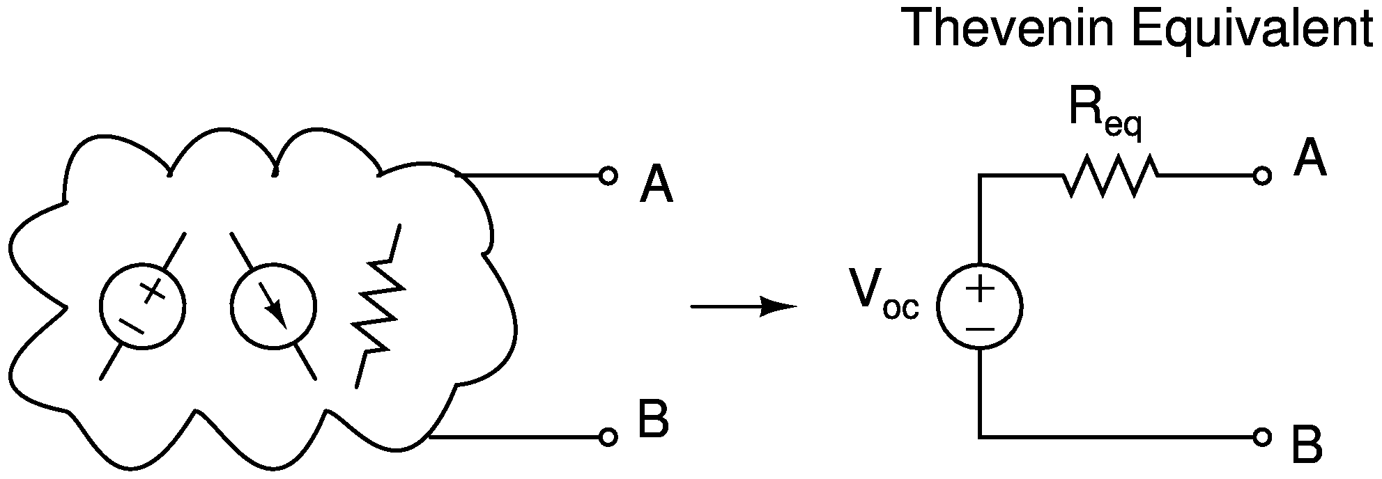
Thévenin’s theorem shows that we can transform any linear circuit comprised of voltage sources, current sources, and resistors from the perspective of any terminal pair A - B, into an equivalent circuit with a single voltage source in series with a single resistor.

Similarly, Norton’s theorem shows that we can transform any linear circuit from the perspective of any terminal pair A - B, into an equivalent circuit with a single current source in parallel with a single resistor.
The Thévenin Equivalent Circuit and Norton Equivalent Circuit are also, of course, equivalent, but different representations of each other.
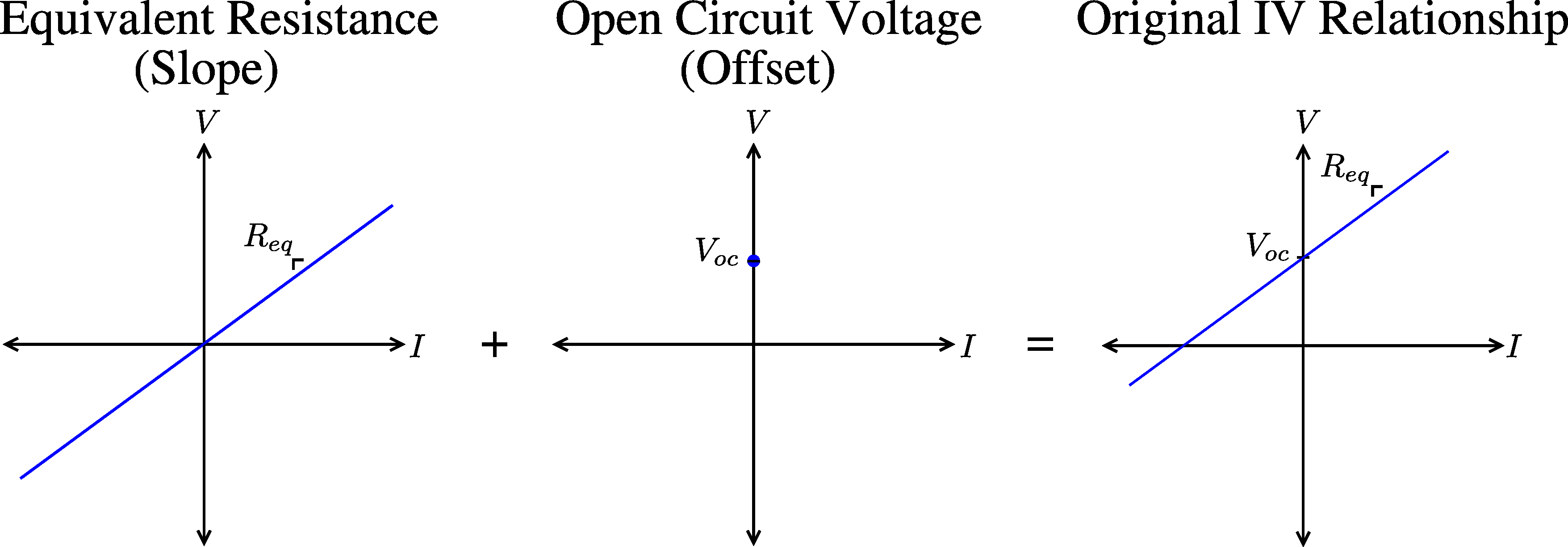
The term “equivalence” here refers to the IV relationship observed at the terminal pair A - B of the linear circuit. For a linear circuit, this relationship will be linear, as in the form y = mx+b:
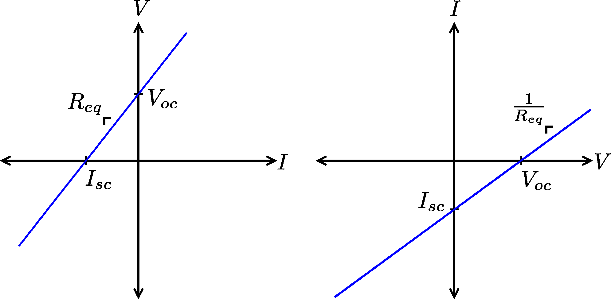
A line is fully characterized by a point on the line and a slope, and in context of an IV relationship, the slope corresponds to the equivalent resistance of the circuit seen across terminals A - B. In the plots above, I’ve labeled the two other relevant points to the Thévenin/Norton equivalent circuits: the open-circuit voltage \( V_{oc} \), that is, the voltage seen across terminals A - B when there is zero current through A - B (an open); and the short-circuit current \( I_{sc} \), that is, the current through terminals A - B when there is zero voltage across A - B (a short).
The Thévenin Equivalent Circuit makes use of the slope \( R_{eq} \) with a resistor, and the offset \( V_{oc} \) with a voltage source, whereas the Norton Equivalent Circuit makes use of the slope \( R_{eq} \) with a resistor, and the offset \( I_{sc} \) with a current source, to model the IV relationship of the original circuit at terminals A - B.
Circuit Tricks
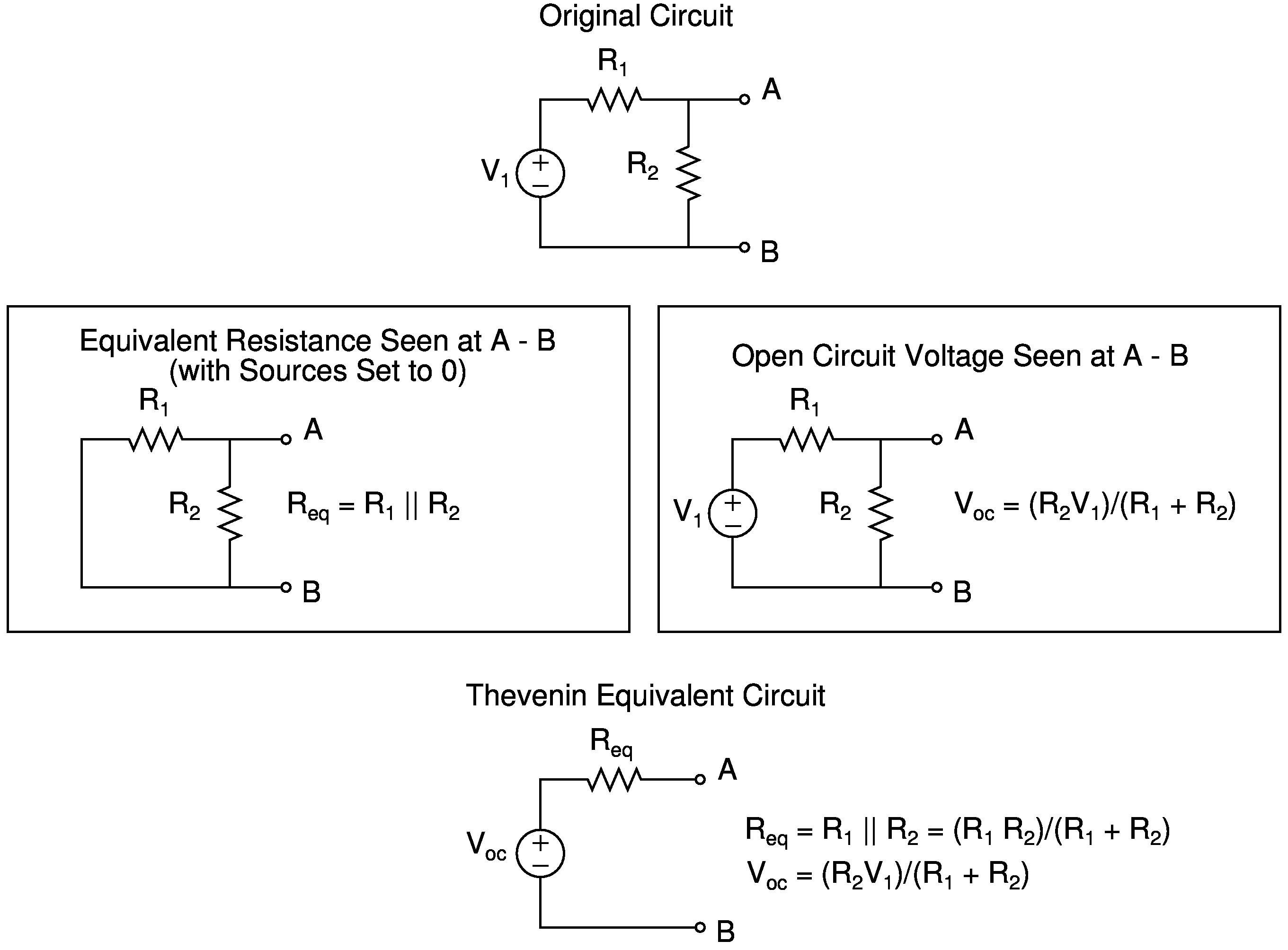
Using circuit techniques, we can find \( R_{eq} \) and \( V_{oc} \) or \( I_{sc} \) with two shortcuts.
- To find \(R_{eq}\), replace voltage sources with shorts and current sources with opens (effectively setting these sources to zero), leaving us with a network of resistors, and then solve for the equivalent resistance seen at terminals A - B.
- To find \(V_{oc}\), solve for the open circuit voltage seen at terminals A to B in the original circuit.
- Alternatively, to find \(I_{sc}\), solve for the short circuit current passing through a short from A to B in the original circuit.
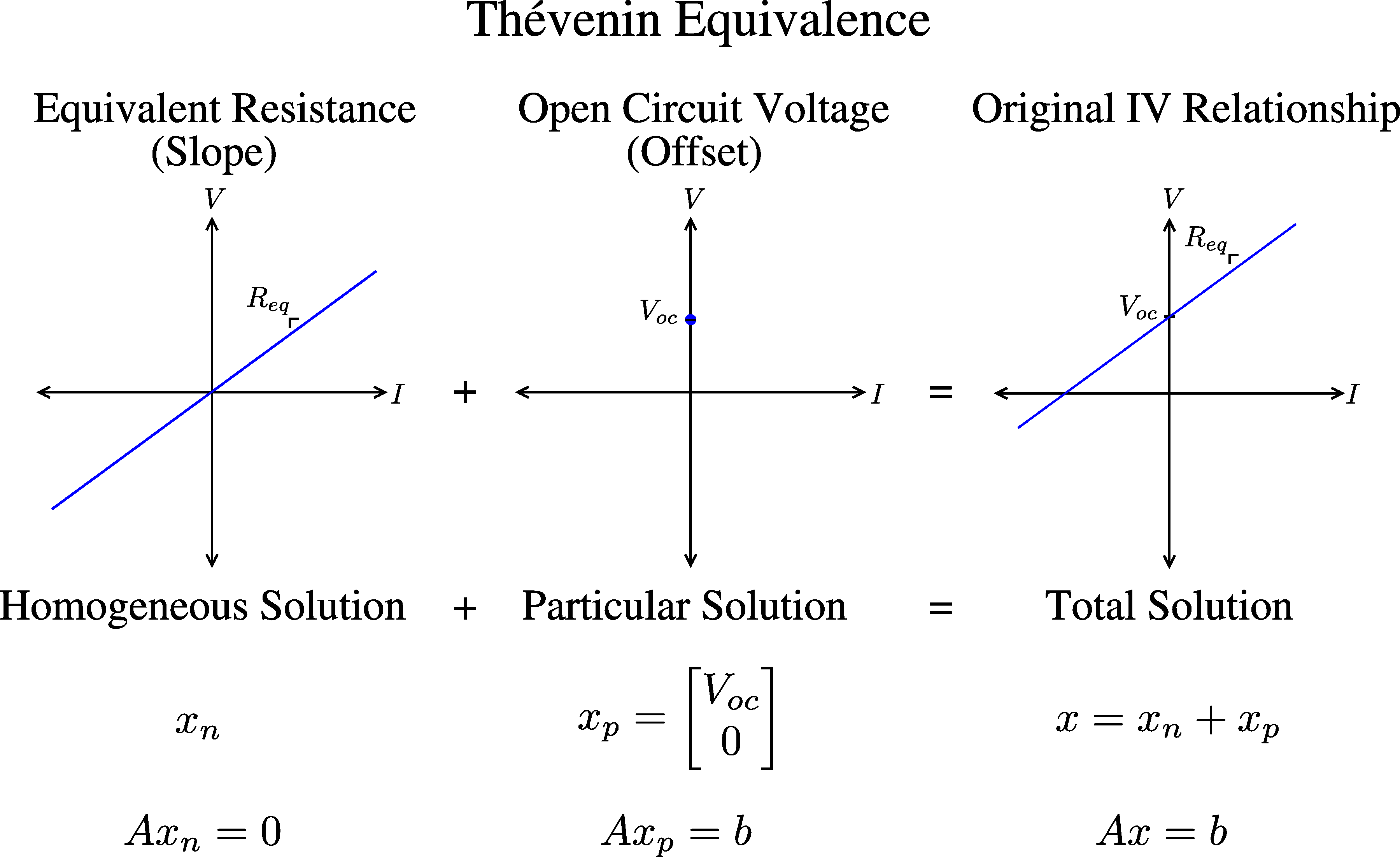
Already, we can see that finding the equivalent resistance gives us a line passing through the origin with the slope of the original circuit’s IV relationship, and finding the open circuit voltage or short circuit current gives us a point from the original circuit’s IV relationship that we can use to translate the line passing through the origin. For example, the Thévenin Equivalent Circuit reconstructs the original circuit’s IV relationship this way:
Linear Algebra Interpretation
Solving for the open circuit voltage and short circuit current made sense to me, but I was always curious about what was actually going on in the process of setting the internal sources to zero and finding the equivalent resistance. So I worked with it a bit, and realized there is a spiffy linear algebra interpretation.
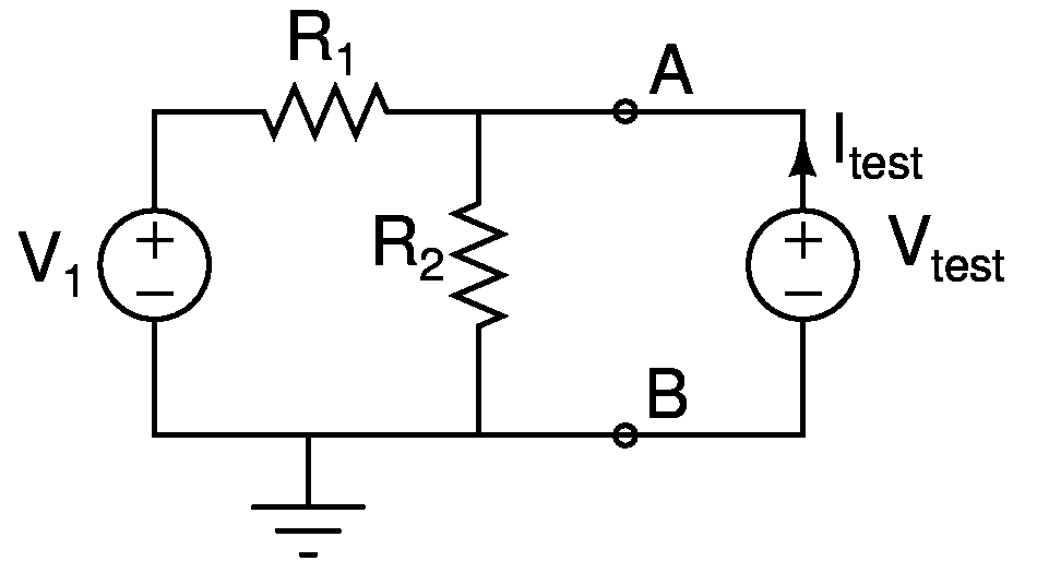
Instead of using the circuit tricks, let’s write out the node equations of this circuit in terms of a hypothetical algebraic test voltage source. Solving for \( I_{test} \) in terms of \( V_{test} \) will give us the IV relationship of the circuit.
\[\begin{eqnarray*} \frac{V_{test}-V_1}{R_1} + \frac{V_{test}}{R_2} - I_{test} = 0 \end{eqnarray*}\]We can rearrange this equation in matrix form, with a matrix of conductances multiplying a vector of the unknowns \( V_{test} \) and \( I_{test} \) on the left side, and a vector of the constant sources on the right side.
\[\begin{eqnarray*} \begin{bmatrix}\frac{1}{R_1} + \frac{1}{R_2} & -1 \\ 0 & 0\end{bmatrix} \begin{bmatrix}V_{test} \\ I_{test}\end{bmatrix} &= \begin{bmatrix}\frac{V_1}{R_1} \\ 0 \end{bmatrix} \end{eqnarray*}\]The conductance matrix here is singular. This makes sense because there are indeed an infinite number of test voltages (plugged into \( V_{test} \)) we can put across terminals A - B that will yield a corresponding current (\( I_{test} \)) and be a solution to the circuit. We know this because the original circuit’s IV relationship is a line.
Now we can relate the two circuit tricks for finding the Thévenin Equivalent Circuit with the above equation in matrix form. To find the equivalent resistance, we first set the internal sources to zero in the circuit trick, which corresponds to setting the vector of constant sources on the right side to zero. Then we can solve the system for \( V_{test} \) and \( I_{test} \):
\[\begin{eqnarray*} \begin{bmatrix}\frac{1}{R_1} + \frac{1}{R_2} & -1 \\ 0 & 0\end{bmatrix} \begin{bmatrix}V_{test} \\ I_{test}\end{bmatrix} &= \begin{bmatrix}0 \\ 0 \end{bmatrix} \end{eqnarray*}\]We are simply solving for the null space, \( Ax_n = \bf{0} \) here! We know that the solution will be a line because the matrix A has two columns and is rank 1, so it must have nullity 1. If we let Wolfram Alpha do the algebra, we arrive at:
\[\begin{eqnarray*} V_{test} = I_{test}\frac{R_1 R_2}{R_1 + R_2} \end{eqnarray*}\]And the relationship between \( V_{test} \) and \( I_{test} \) here is precisely the equivalent resistance we solved for in the previous section: \( R_{eq} = \frac{R_1 R_2}{R_1 + R_2} \).
Now let’s carry out step two of the circuit tricks for finding the Thévenin Equivalent Circuit. This is finding the open circuit voltage at terminals A - B (where we have our hypothetical test voltage source \( V_{test} \)). For this step, we solve the circuit with our hypothetical test voltage source and zero current flowing through it, that is, we constrain \( I_{test} = 0 \).
\[\begin{eqnarray*} \begin{bmatrix}\frac{1}{R_1} + \frac{1}{R_2} & -1 \\ 0 & 0\end{bmatrix} \begin{bmatrix}V_{test} \\ 0\end{bmatrix} &= \begin{bmatrix} \frac{V_1}{R_1} \\ 0 \end{bmatrix} \end{eqnarray*}\]Once again, if we let Wolfram Alpha do the dirty work, we get:
\[\begin{eqnarray*} V_{test} = V_1 \frac{R_2}{R_1 + R_2} = V_{oc} \end{eqnarray*}\]Here we’ve simply solved for a particular solution \( Ax_p = b \), and got exactly the open circuit voltage \( V_{oc} = V_1 \frac{R_2}{R_1 + R_2} \) we solved for in the previous section.
Alternatively, we could have chosen the constraint \( V_{test} = 0 \), and solved for \( I_{test} \):
\[\begin{eqnarray*} I_{test} = -\frac{V_1}{R_1} = I_{sc} \end{eqnarray*}\]This is another perfectly valid particular solution, and is the short circuit current \( I_{sc} \) that the Norton Equivalent Circuit uses in its representation of the circuit. In fact, we can use any fixed value constraint on either \( V_{test} \) or \( I_{test} \), to solve for a particular solution, but these choices of \( I_{test} = 0 \) or \( V_{test} = 0 \) have convenient circuit representations.
From linear algebra, we know that the general solution to \( Ax = b \) is \( x = x_n + x_p \). In words:
Total Solution = Homogeneous Solution + Particular Solution
We can add the homogeneous solution and the particular solution above to yield:
\[\begin{eqnarray*} V = I \frac{R_1 R_2}{R_1 + R_2} + \frac{R_2 V_1}{R_1 + R_2} = I R_{eq} + V_{oc} \end{eqnarray*}\]or:
\[\begin{eqnarray*} I = V\frac{R_1 + R_2}{R_1 R_2} - \frac{V_1}{R_1} = V\frac{1}{R_{eq}} + I_{sc} \end{eqnarray*}\]These are exactly the simple decompositions that the Thévenin/Norton theorems deliver. We can easily model the first equation with a circuit of a constant voltage source in series with a resistor (the Thévenin equivalent), and we can model the second equation with a circuit of a constant current source in parallel with a resistor (the Norton equivalent).
So the Thévenin/Norton equivalent “circuit tricks” correspond exactly to finding the homogeneous and particular solutions at terminals A - B of the original circuit.
The “circuit trick” for setting the internal sources to zero and finding the equivalent resistance is just finding the homogeneous solution to the original circuit at terminals A - B, and is represented by a resistor in the equivalent circuit. This makes sense, since a resistor models the solution to the null space (a line) by imposing a linear constraint at the terminals A - B. Finding the open circuit voltage or short circuit current is just finding a particular solution, and this is represented by a constant source in the equivalent circuit. This also makes sense, since a constant source models the constant offset that translates the homogeneous solution.
Now we can augment our previous picture with this interpretation: