Windowing in a Nutshell

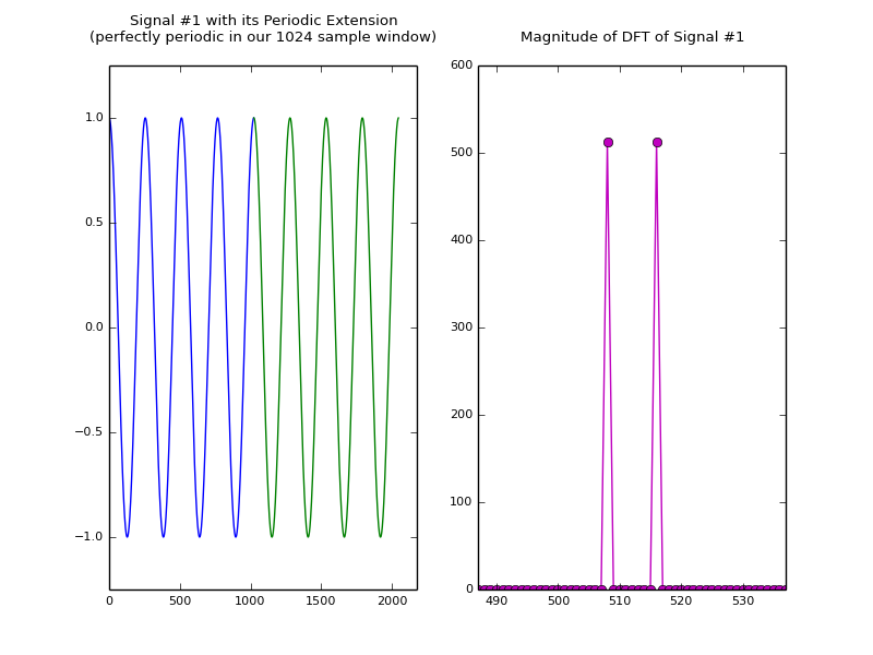
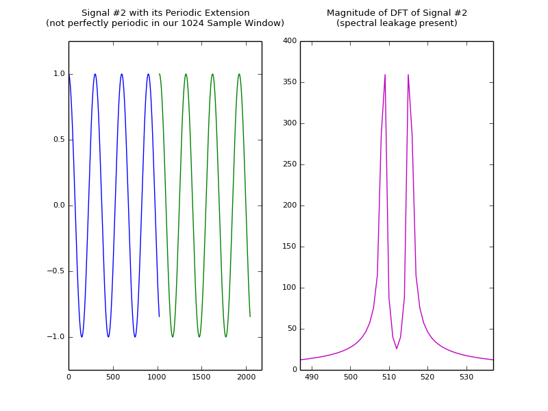
The DFT operates on a finite duration signal, and assumes an infinite periodic extension of that signal. If your signal is not periodic in the sample window you are evaluating the DFT with, you will see frequency components associated with the time domain discontinuity of the periodically extended signal (also called spectral leakage). You can use a window function to taper off the beginning and end samples of the signal, so that these time domain discontinuities are minimized and the DFT of it is a better representation of the frequency content in the actual signal.

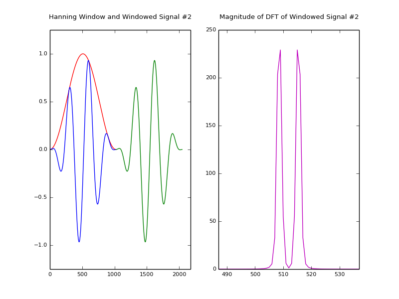
Applying a window is easy:

w = np.hanning(len(sig))
wsig = sig*w

Code for the plots above:

import numpy as np
import scipy.signal
import pylab

pylab.rc('font', **{'weight': 500, 'size': 8})

# Signal #1, perfectly periodic in t=0,...,1023
t = np.arange(0,1024);
y = np.cos(2*np.pi*t/256.0)

# Plot Signal #1 and its periodic extension
pylab.subplot(121)
pylab.plot(t, y)
pylab.plot(t+1024, y)
pylab.axis([0, 2048+128, -1.25, 1.25])
pylab.title("Signal #1 with its Periodic Extension\n" \
    "(perfectly periodic in our 1024 sample window)\n")

# Plot Magnitude of DFT of Signal #1
pylab.subplot(122)
pylab.plot(np.abs(np.fft.fftshift(np.fft.fft(y))), '-om')
pylab.xlim([512-25, 512+25])
pylab.title("Magnitude of DFT of Signal #1\n")
pylab.savefig('windowing_nutshell_1.png')
pylab.show()

pylab.clf()

# Signal #2, not perfectly periodic in t=0,...,1023
y = np.cos(2*np.pi*t/300.0)

# Plot Signal #2 and its periodic extension
pylab.subplot(121)
pylab.plot(t, y)
pylab.plot(t+1024, y)
pylab.axis([0, 2048+128, -1.25, 1.25])
pylab.title("Signal #2 with its Periodic Extension\n" \
    "(not perfectly periodic in our 1024 sample window)\n")

# Plot Magnitude of DFT of Signal #2
pylab.subplot(122)
pylab.plot(np.abs(np.fft.fftshift(np.fft.fft(y))), '-m')
pylab.xlim([512-25, 512+25])
pylab.title("Magnitude of DFT of Signal #2\n" \
        "(spectral leakage present)\n")
pylab.savefig('windowing_nutshell_2.png')
pylab.show()

pylab.clf()

# 1024 point Hanning Window applied to our Signal
w = np.hanning(1024)
yw = y*w

# Plot Hanning Window, Windowed Signal #2,
# and its periodic extension
pylab.subplot(121)
pylab.plot(t, w, 'r')
pylab.plot(t, yw, 'b')
pylab.plot(t+1024, yw, 'g')
pylab.axis([0, 2048+128, -1.25, 1.25])
pylab.title("Hanning Window and Windowed Signal #2\n")

# Plot Magnitude of DFT of Signal #2
pylab.subplot(122)
pylab.plot(np.abs(np.fft.fftshift(np.fft.fft(yw))), '-m')
pylab.xlim([512-25, 512+25])
pylab.title("Magnitude of DFT of Windowed Signal #2\n")
pylab.savefig('windowing_nutshell_3.png')
pylab.show()

Comments